

Google Sheets: Best Practices for Ops
Pro Tips for Ops on Google Sheets, Part 1

Welcome to the 5 new Ops Hackers that have joined us since last week! We’re currently 7 Ops Hackers strong :)
We ❤️ Google Sheets
This week, I want to return to basics and talk about the one tool that every ops person spends a disproportionate amount of time on: Google Sheets. Let’s be honest - we use it for everything from project management to dashboards.
For the record, I recognize that Google Sheets is necessarily the best tool for everything that I use it for, but I find myself return to it week in and week out because of how comfortable I am with the tool. I once tried to use Google Sheets to create an internal task management tool that scheduled and assigned chores to team members. The maintenance and constant re-jigging of the tool took way too much time and eventually it was scrapped. If you search hard enough or know where to look, there’s usually an ideal tool out there for what you’re trying to accomplish, especially in this day and age where there’s a SaaS for every use case. As I continue to expand and build out my tool stack, I’m going to share everything I learn with you, so you hopefully don’t have to sit through product demos / climb up the learning curve for every tool. Or try to shoehorn Google Sheets into building a productivity tool. But I digress.
Given Google Sheets’ prominence in an ops tool stack, I think it’s worthwhile going through some best practices that will help you and co-editors of your sheets. This isn’t an exhaustive list by any means, but rather a shortlist of best practices that I’d share with new ops people on my team. So the list assumes at least a base level understanding of Google Sheets.
Some or possibly all of these tips I’m about to share might be obvious to you - but hopefully you’ll learn something new and if not, at the very least, this post will serve as a reminder to continue practicing good sheet habits.
Today’s post is the first part of a 2-part series in which I’ll discuss my Google Sheets best practices (part 1) and personal favourite functions (part 2).
1. Colour code your cells
If I’m being honest with myself, I didn’t really enjoy my time working in banking. But I’m grateful for everything I learned during those years, especially around Excel. As you may already know, investment banking analysts spend a lot of time building financial models in Excel. And one of the first things you learn is to colour code your cells.
Colour coding is really important from a User Experience (UX) perspective. It quickly tells the viewer of a sheet which cells are formulaic vs. hardcoded, and which cells are okay to play around with vs. should be left alone. This saves you, the creator of the sheet, a ton of time as it minimizes the amount of explanation you have to do to others who want to use your sheet.
Every bank has a slightly different colour coding convention and mine’s evolved since my banking days, but here’s mine:
Black: Formula
Blue: Hardcoded value
Green: A formula referencing another sheet in the same file
Brown: A formula referencing another file (using the importrange function)
Yellow background: A cell requiring an input value from the user
See screenshot below for a visual explanation of this convention.
2. Include a legend
Just in case someone who’s looking at your sheet doesn’t understand your colour coding convention, include a legend as a sheet outlining what colours mean what. This is helpful especially when the sheet gets shared outside of your group. It’s easy to create this sheet once and then copy and paste it into other sheets you create in the future.

Here’s an example of mine that you can copy and use if you’d like.
3. Utilize Custom Number Formats
You can access Custom Number Formats by going to Format > Number > More Formats > Custom Number Format.
When you go into Custom Number Format, you see a window like this:

The highlighted text above may look liked jumbled characters, but it follows a certain convention:
positive; negative; zero; textThe semicolon acts as a separator between the four types of values and how you’d like each of them formatted.
The formatting in the above screenshot is telling Google Sheets to include a comma as a thousands separator, show one decimal point, use parentheses to indicate a negative value (more legible than a minus symbol), and for non-negative values to add a space equal to a parenthesis so all the values line up nicely when right-aligned.
With using brackets in custom number formatting, you can even do things like this:
[<25]"Small";[>=25]"Large";"Other"This formatting would show “Small” for any value under 25, “Large” for 25 and over, and “Other” for other values (i.e. non-numerical values). You could achieve a similar output by using an if function (i.e. if(value<25, “Small”,…), but the difference here is that you’re just formatting the external appearance of the value and not changing the actual underlying value; so unlike an if function, you could still execute numerical operations on values that appear as “Small” or “Large”.
Here’s a deeper dive on custom number formatting by Ben Collins that explains the concept really well with various examples.
4. Name your favourite cells
If you’re ever building a fairly complex model or dashboard, make sure to name the cells that get used often (Data > Named Ranges).

Perhaps you have a scenario picker that toggles between bull, base, and bear cases in cell A2 in sheet “scenario”. You’ll likely have to repeat writing out “scenario!A2” a lot as you’ll continue to refer to this cell to build out your three scenarios. In this case, assign a name to the cell - something like “case” to indicate the three cases.
Now you can write your formulas much more quickly by referencing “case”. And you can start writing a much easier-to-understand formulas like this:

5. Use keyboard shortcuts
If you spend a not-insignificant amount of time in Google Sheets, you should invest some time to ramp up on keyboard shortcuts. They will save you a ton of time eventually.
For example, to access the Custom Number Formatting menu in section 3 by mouse, it took me 8 seconds. But the keyboard shortcut of Ctrl + Option + O > N > O > up arrow > enter takes less than a second once it’s in your muscle memory.
Here’s a full list of shortcuts available on Google Sheets. I recommend you print it out and put it next to your computer screen. At first, using keyboard shortcuts will be slower than using your mouse. But gradually as you start memorizing them, you will see a vast improvement in your speed. (This principle of using keyboard shortcuts over a mouse applies to any tool that you use often enough.)
An easy way to get ramp up on keyboard shortcuts in Google Sheets is to start with memorizing just the following:
File menu: Ctrl + Option + f
Edit menu: Ctrl + Option + e
View menu: Ctrl + Option + v
Insert menu: Ctrl + Option + i
Format menu: Ctrl + Option + o
Data menu: Ctrl + Option + d
Tools menu: Ctrl + Option + t
When you use these shortcuts to access a menu, Google Sheets is smart enough to realize you are a “hotkeys person” and shows you keyboard shortcuts for actions inside the menu:
When you use a mouse to access the View menu:

When you use a keyboard shortcut to access the View menu:

6. Navigate using “elevator cells”
“Elevator cells” are cells that I use to jump quickly up and down a sheet. You can build your sheet in a certain way to allow for a quicker navigation. Here’s an example:

I’ve illustrated what an operational model’s headers might look like in this example. You can see that there are two major sections, Scenarios and Summary, and the latter has sub-sections like KPIs and Financial Snapshot. Instead of using indentation within the cell, I’m actually using an array of different columns to show the hierarchy. In other words, column B is being used to show the major sections (Scenarios in cell B2 and Summary in B7) while column C is being used to show the sub-sections (KPIs in cell C8 and Financial Snapshot in cell C17).
If I wanted to move from KPIs (cell C8) to Financial Snapshot (cell C17), I could hit the down arrow on my keyboard 9 times (or try to use my mouse), but I can also hit command + down arrow, which is a keyboard shortcut that takes me down to the next non-blank cell or cell C17 in this case.
Nothing groundbreaking here, but once you learn how to navigate Sheets using keyboard shortcuts, you can incorporate this knowledge in how you design and structure your sheets which further improves your productivity with Sheets.
7. Distinguish between data, input, and output
More often than not, you’re not the only one with access to your sheet. You’ve probably shared the sheet with your team and manager, and they might have shared it with other people. To make sure that others don’t inadvertently break your sheet and also to help them navigate your sheet more easily, you should make it clear what’s raw data, what requires their input, and what is the output.

You can do this by keeping these three components in their separate sheets. I like to keep my raw data in a sheet named “raw”, input in a “main” sheet, and output in a sheet called “output” or “charts” depending on what type of output it is, like this:

You can also make sure no one else can edit your raw and output sheets by putting a sheet protection on them (Tools > Protect Sheet). And you can take it even one step further by hiding the protected sheets (right click on the sheet tab and select Hide sheet) - this helps viewers focus on what you want them to see in your sheet by removing other distractions.
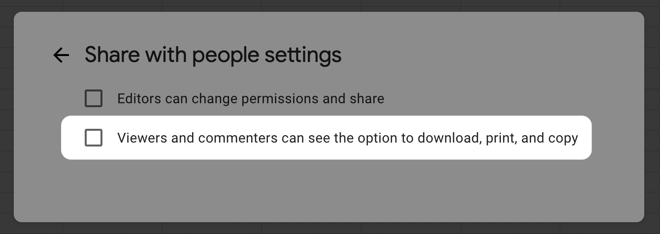
By the way, if a person has an edit access, they can unhide hidden sheets. And even if they only have a view access (vs. an edit access) to your sheet, they’ll still be able to see what’s in the hidden sheet if they have a download, print, and copy access - by making a copy of your file.
8. Write scalable formulas
You probably already know that when you’re referencing a range of cells, you don’t need to specify the ending row to capture all the rows, i.e. instead of writing sum(A1:A1000), you can write sum(A1:A) which will capture all the rows in column A beyond a thousand.
But did you know you could do the same with columns? So instead of entering sum(A1:Z1), you can write sum(A1:1).

This “un-specifying the end row/column” helps keep your sheet more scalable, because you can continue to add more data in the future without having to go back to pre-written formulas to capture newly added columns and rows.
In Part 2 of our deep dive into Google Sheets, I’ll walk through some specific functions that help ensure scalability of your sheet.
9. DRY
"Don't repeat yourself" (DRY, or sometimes "do not repeat yourself") is a principle of software development aimed at reducing repetition of software patterns, replacing it with abstractions or using data normalization to avoid redundancy.
Source: Wikipedia
You could argue that working with data in Google Sheets is a form of software engineering, and I’d say the DRY principle definitely applies as well.
I’ve seen a lot of sheets that have the same data duplicated in multiple places. Perhaps you’re pulling in raw data of your driver sign-ups into a couple different places to: 1) create a forecast model and 2) build a KPI dashboard of sign-ups so far. As soon as you start manipulating either the data in #1 or #2 but not the other, you will have two sets of data that are supposed to be identical but no longer are. And you’ll get different values depending on which data set you reference. This is especially problematic if you aren’t referencing the original source (the raw data in this case) in a formula but instead copying and pasting values somewhere.
 | Make a Meme")
The easiest way to ensure you D.R.Y. is minimizing hard-coding. Restrict the amount as well as the location of your hardcoded / raw data, and everything else should be a formula that refers back to your hard data.
Takeaways
We covered 9 basic best practices in using Google Sheets:
Colour code your cells
Include a legend
Utilize Custom Number Formats
Name your favourite cells
Use keyboard shortcuts
Navigate using “elevator cells”
Distinguish between data, input, and output
Write scalable formulas
DRY
In the next post, I will walk you through some of my personal favourite functions in Google Sheets.
As always, please let me know what you thought of this by leaving a comment below or email me at hi@joerhew.com :)
Love this! I didn't know you could go that deep with custom number formatting! I'll definitely add this to my workflow - Thanks Joe!
I enjoyed this one. Very practical tips.