

Google Sheets for Ops: Logical Functions
Pro Tips for Ops on Google Sheets, Part 2

Welcome to the 24 new Ops Hackers that have joined us since last week, bringing the grand total to 31! :)
Fun Functions
So I know last week I said this post will be Part 2 of 2 where I’ll share my favourite Google Sheets functions. As I sat down and started writing out the different functions that’s helped me navigate ops at Uber and other startups, I realized that there’s way too many to cover in one email.

So I’m calling a last minute audible to make this into a multi-part series instead:
In Part 1, we covered some Best Practices when using Google Sheets.
In Part 2 (this email), we’ll cover logical functions.
In Parts 3 and beyond, we’ll cover text, lookup / data, date, and miscellaneous functions.
For Parts 2 and onward, I’m creating example spreadsheets that you can make a copy of to follow along. You can find this week’s spreadsheet here:
Follow along this week’s Google Sheets function examples in this sheet.
To illustrate how the functions work in real life, we’ll be using Kaggle’s dataset on public data on Airbnb listings in New York City from 2019, found here. I’ve copied the first 2,000 rows into the example sheet, in the “raw_data” tab.
What’s a logical function?
A logical function in Google Sheets returns either a True or a False value depending on whether the logical expression you feed to it is true or not. One logical function that everyone should be familiar with is IF: you write a logical expression and tell Google Sheets to give you value 1 if the IF statement is true, and value 2 if the statement is false.
With that definition, let’s get started with our first logical function.
1. IFS
Everyone knows about the IF function, but not everyone knows about IFS. The IF function’s logic goes like this:
=IF(logical_expression, value_if_true, value_if_false)The IF function is great if there is only one logical expression, such that there are only two outcomes, true or false. However, if there are multiple logical expressions, the formula can get messy real quick with a lot of nested IFs, like:
=IF(logical_expression_1, value_if_true, IF(logical_expression_2, value_if_true, IF(logical_expression_3, value_if_true, value_if_false)))This is where IFS comes in handy. IFS’s logic handles multiple logical expressions in a more comprehensible way:
=IFS(condition1, value1, [condition2, …], [value2, …])So instead of writing a formula like

You can increase the legibility by writing:

The IFS function can help you understand others’ (and your own) spreadsheet more quickly, as well as reducing errors related to incorrectly nested logic. The rule of thumb in deciding whether to use IFS over IF is “always use IFS unless there are no nested IF statements”.
Note that the IFS function evaluates each logical expression sequentially and stops immediately after finding a true logical expression. So the order in which you write out your logical expressions is important.
For example, in the IFS statement above, the second-to-last logical expression:output value pairing is $c11>0:”1-100”. If this pairing’s position was ahead of "$c11>300:”301-364” in the formula, the output value for any number between 301 and 364 would be “1-100”, and not “301-364” as we intended. This is because technically any number between 301 and 364 is greater than 0 (i.e. logical expression is true), and Google Sheets stops evaluating the rest of the logical expressions. I know it’s a bit confusing, but compare the formulas in cells D11 (correct order of logical expressions) and E11 (reversed order) in this sheet, and it should be clear.
Here’s an example comparing IF to IFS.
2. AND / OR
AND and OR functions come in handy when you are trying to construct complex logical arguments in combination with IF and IFS.
The AND function is only true if all of the logical arguments nested inside the function are true, and denoted as:
=AND(logical_expression_1, logical_expression_2, ...)The OR function is true if any of the logical arguments are true.
=OR(logical_expression_1, logical_expression_2, ...)When you combine these functions, you can create powerful logical queries like:
=IF(AND(OR(C7="Manhattan",D7="Williamsburg"),E7<200),"YES","")
In plain English, the above formula is saying:
If the listing’s neighbourhood_group is Manhattan OR neighbourhood is Williamsburg AND its price is below $200, mark the listing as a “YES”; otherwise, leave blank.
Listing ID 2539 doesn’t meet the criteria because it’s in Brooklyn (not Williamsburg), and neither does ID 2595 because its price is over $200. ID 3647 is in Manhattan and the price is below $200, so it gets a “YES”.
3. SWITCH
The SWITCH function evaluates an expression and returns one of multiple values which are pre-set by you. This function is similar to IFS in that there are multiple outcomes based on an evaluation. The main difference is that in IFS, you’re evaluating a logical expression and returning a value if that logical expression is true; in SWITCH, you’re evaluating an expression with multiple outcomes and returning a value based on it1. The syntax for the SWITCH function is:
=SWITCH(expression, case1, value1, case2, value2, ..., default)This function is much easier to understand with an example:

In the above example, I wrote a formula that evaluates the neighbourhood of a listing and assign a rating based on which neighbourhood it’s in. Note that I’m not evaluating whether the listing is in a certain neighbourhood, because that would be a logical expression and I’d be better off using the IFS function instead. Below are the neighbourhood-rating pairings:
Good: Hell’s Kitchen and Midtown
Great: Murray Hill and Bedford-Stuyesant
It’s still NYC!: Everywhere else
The last pairing for everywhere else is the default or fallback value for SWITCH that it reverts to if the expression it is evaluating doesn’t match any of the specified pairings. Note that unlike SWITCH, the IFS function doesn’t have a default value. For example, we didn’t assign a rating to Kensington, so listing ID 2539 defaults to “It’s still NYC!”

4. IFERROR / ERROR.TYPE
IFERROR is a shorthand function that is equal to IF(ISERROR(value)). It evaluates a value and displays it if it’s not an error; if it is an error, it either shows the cell as a blank (default) or another value if you specify it. Here’s the syntax for IFERROR:
=IFERROR(value, [optional_value_if_error])Below is an example that shows Month-over-Month revenue growth. In the “MoM Revenue Growth %” row (unhighlighted), you can see two errors: #VALUE! and #DIV/0!. The #VALUE! error is due to trying to get the growth rate for the first month (i.e. dividing $3,000 in cell C5 by the text value “Monthly Revenue” in cell B5). The #DIV/0! error is because I’m trying to divide $8,000 by zero.
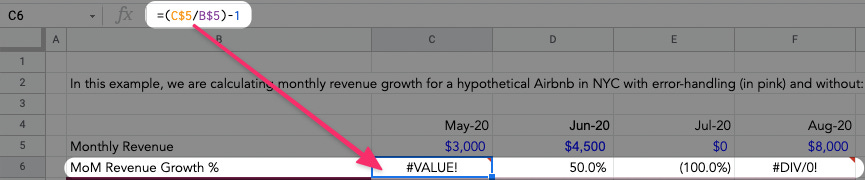
These error values are problematic, because any subsequent calculations involving them also result in an error value. They are also distracting and look unprofessional.
You can clean up these errors by using IFERROR:

Now there are blanks instead of error values because I wrapped an IFERROR function around the expression. I could have also opted to show a custom error message like “ERROR” by including the optional value like this:
=IFERROR(C$5/B$5-1,"ERROR")Or…I could make it really fancy by showing different error messages based on the type of error by using ERROR.TYPE.
What’s an ERROR.TYPE?
There are 8 different error types in Google Sheets. Going into each feels out of scope for this post, but you can refer to this excellent writeup by Info Inspired to learn more.

For the purposes of this post, we can combine what we learned in SWITCH with ERROR.TYPE to show different messages based on the error, like this:
In plain English, the formula above is saying:
Show the MoM growth rate by dividing this month’s revenue by the previous month’s revenue and then subtracting 1. If there is an error, get the error type. If the error type is 2 (i.e. #DIV/0!), then show “Prev month was $0”. If the error type is 3 (i.e. #VALUE!), show “First month”. For all other errors, show a generic error message “Error - check formula”.
5. ISBLANK
Remember how I said IFERROR = IF(ISERROR(expression))? ISBLANK is like ISERROR, but it evaluates whether a cell is blank or not and returns a true / false value. I use ISBLANK in combination with IF (or IFS) a lot, because Google Sheets doesn’t have an IFBLANK function. So you have to write out IF(ISBLANK(expression)) unlike IFERROR.
ISBLANK is super useful, because calculations involving blank cells do not result in an error (unlike zero or text values). But there are times when you want to treat blank values differently to avoid inadvertently making mistakes in your calculation. Let’s use the revenue growth example from the previous section to illustrate this point. If we’re launching a marketing campaign and expect our MoM growth rate to increase by 2x:
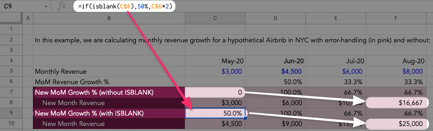
Recap: Our MoM revenue growth for the first month was causing an error in the previous section so we used the IFERROR function to show a blank cell instead. Now, when we multiply that blank cell by 2, the new value will be 0 (cell C7) because Google Sheets treats blank cells like zeros. To account for the marketing campaign’s impact, we can instead write a formula to hardcode a growth rate (50% in this case) like this:
=IF(ISBLANK(C6),50%,C6*2)This ensures that we’ll either 2x the previously stated growth rate or if the cells is blank, assume the growth rate will be 50%. As you can see in the screen capture above, the resulting new monthly revenues can differ quite a lot ($16,667 vs. $25,000) depending on whether you’ve accounted for blank values.
Takeaways
In this post, we covered logical functions in Google Sheets that ops should know:
IFS: We talked about when to use IFS over IF (i.e. when there are multiple logical expressions).
AND / OR: We covered how to combine AND or OR functions together with IF statements to build complex logic into our formulas.
SWITCH: We learned about the SWITCH function, which is similar to IFS except it handles expressions that could output multiple values vs. a logical expression which has only 2 possible values.
IFERROR / ERROR.TYPE: We explored the IFERROR function and how we can use it to get ahead of any errors that may occur in Google Sheets. We briefly touched on the ERROR.TYPE function as well and how we could use it to customize our error messages.
ISBLANK: Lastly, we introduced the ISBLANK function, which is often used together with an IF statement, and discussed why it’s good practice to write a formula that handles blank values when you’re working with Google Sheets.
If you’re interested in learning more on your own, here’s a comprehensive list of all Google Sheets functions.

In the next post, we’ll dive further into more functions, starting with text functions that will make your life easier if you work with a lot of text values.
As always, please let me know what you thought of this by leaving a comment below or email me at hi@joerhew.com :)
So technically, SWITCH is not a true logical function. But I’m including it in this post because it shares a lot of similarities with the IFS function.
Never used SWITCH before, I’ll try it out :)